RoboMaster Wheel-Legged Robot – Dynamics & Control

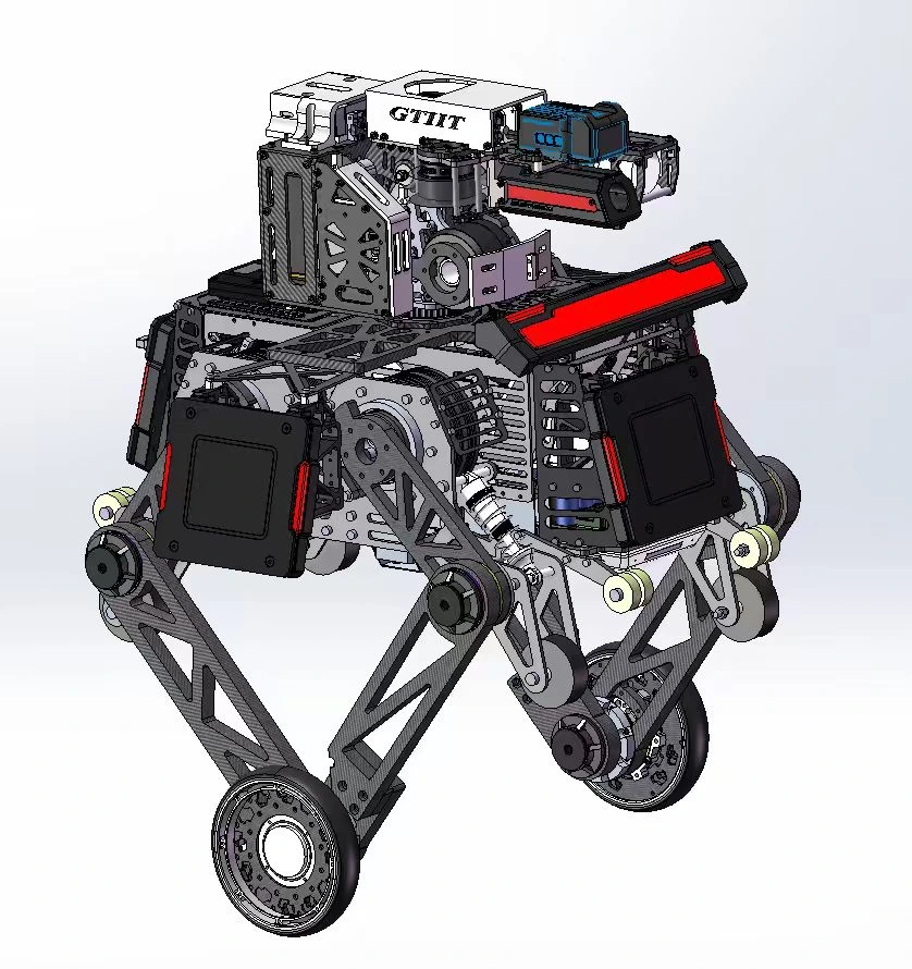
As a member of the Electrical Control Group in GTIIT’s RoboMaster KongFu Team, I contribute to embedded robot control and control-algorithm development.

This selected project focuses on the dynamics and balance control of a wheel-legged chassis. My work connects five-bar kinematics and virtual model control with a leg-length-dependent LQR controller, followed by nonlinear MATLAB/C validation of recovery and tracking.

Role: Electrical Control Group Member
Technical focus: Embedded Control · Robot Dynamics · Feedback Control

View validation repository Explore simulation evidence

Isometric CAD view of the RoboMaster wheel-legged robot showing the chassis, five-bar legs, and wheels — Team-provided robot CAD assembly. The wheel-legged platform is the selected system for my control work.

My role

Control & algorithm development

Wheel–leg–body dynamics and leg-length-dependent LQR feedback.
Five-bar kinematics, Jacobians, and virtual model control in C.
Nonlinear MATLAB/C validation of recovery, tracking, and model-parameter sensitivity.

Team-provided foundation

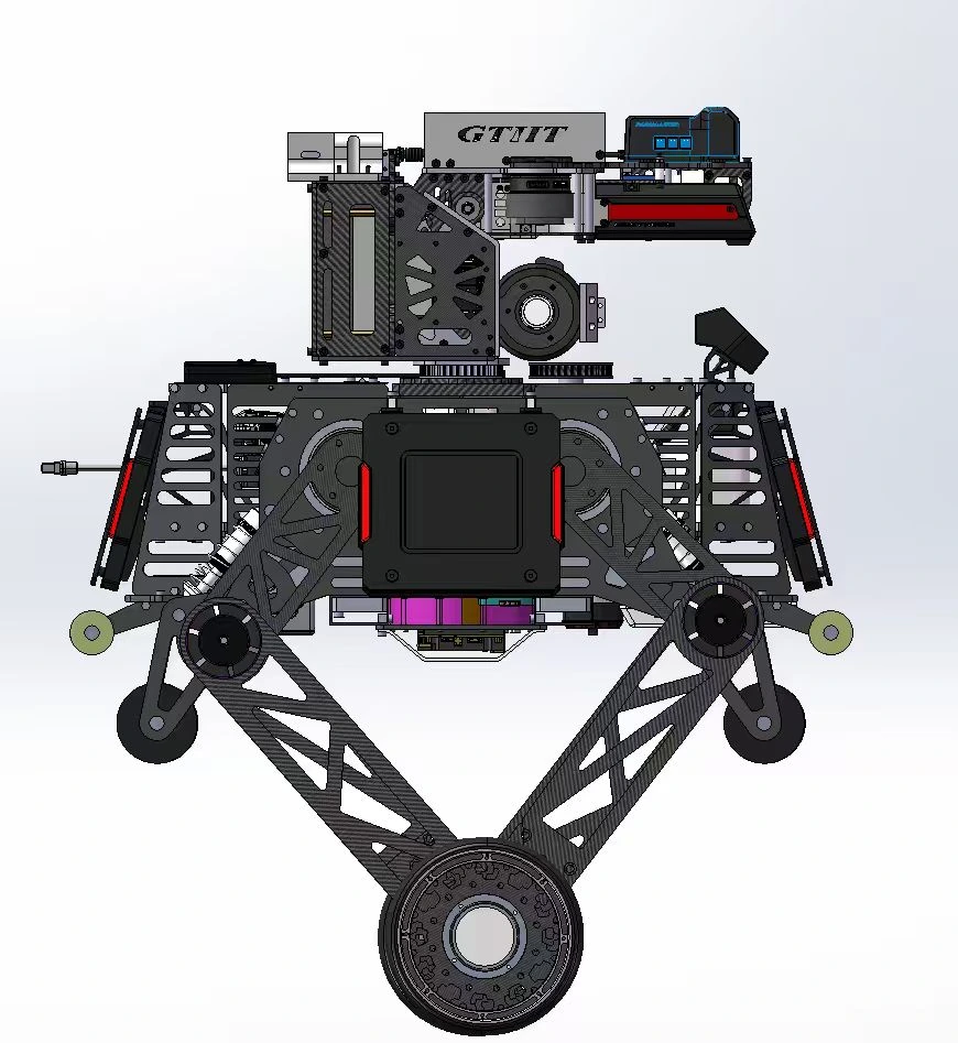
The mechanical platform, CAD inputs, and historical control-code base come from the team project. The maintained C modules retain that lineage; the validation repository records their provenance alongside the later simulation work.

6 statesWheel–leg–body balance modelLeg angle, longitudinal motion, body pitch
11 nodesLeg-length-dependent LQR gainsInterpolated over 0.1042–0.3672 m
600 trialsModel-parameter uncertainty study100 samples × 3 fixed lengths × 2 controllers

Control architecture

The control stack connects mechanism geometry to virtual leg forces, wheel–leg–body dynamics, and state feedback. A nonlinear plant then exercises the maintained C balance controller through MATLAB MEX.

Five-bar kinematics & virtual model control

The five-bar linkage maps two driven joint angles to an equivalent leg length and angle. I worked on forward/inverse kinematics and Jacobian-based virtual model control in C, with workspace and singularity checks before mapping desired forces and moments to joint torques.

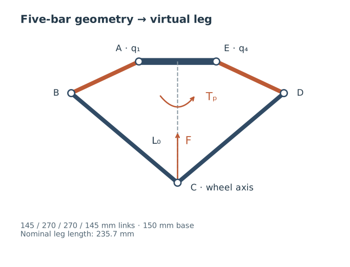
Side CAD view showing the body above the articulated five-bar leg and wheel — Side view of the assembly. The control abstraction retains body pitch, equivalent leg angle, and wheel motion.

Five-bar diagram derived from CAD parameters: driven pivots A and E, passive joints B and D, wheel axis C, virtual axial force F and hip moment Tp — Code-derived geometry at L₀ = 0.2357 m. Link lengths and the 0.15 m pivot spacing come from the validation repository's CAD parameters.

For J = ∂(L₀, α)/∂(q₁, q₄), virtual work gives the force-to-torque relation:

τ = Jᵀ [F, Tₚ]ᵀ

Dynamics, LQR & gain scheduling

The six-state model couples equivalent leg angle θ, longitudinal displacement xᵦ, and body pitch φ with their rates. Per-side wheel torque T and virtual hip torque Tₚ regulate body balance and longitudinal motion.

x = [θ, θ̇, xᵦ, ẋᵦ, φ, φ̇]ᵀ

u = [T, Tₚ]ᵀ = K(L₀)(x_ref − x)

Configuration-dependent dynamics motivate a leg-length-dependent feedback matrix. The implementation interpolates a 2 × 6 matrix between 11 nodes; the nominal 0.2357 m gain provides the fixed-gain comparison used below.

0.1042 mNominal · 0.2357 m0.3672 m

C implementation in the nonlinear simulation

The MEX interface executes the maintained C FiveBar/LQR path inside MATLAB. Independent MATLAB references check geometry, gains, and commands, connecting the control derivation to the implementation being tested.

01 · Reference & sensingState error
Reference minus the ideal state measurement, with C five-bar geometry.
02 · C controller via MEXK(L₀) feedback
Interpolated gains produce wheel and virtual hip torque requests.
03 · MATLAB plantNonlinear response
Limited torques advance the fixed-length half-car model; state feeds back to step 01.

VMC is implemented and separately tested. The closed-loop studies below apply generalized T and Tₚ directly to the plant, so their scope ends before the full joint-actuator dynamics.

Simulation validation

The studies test recovery, disturbance rejection, velocity tracking, and sensitivity to model uncertainty across fixed leg configurations. Gain scheduling changes the performance tradeoffs across lengths. Select a plot to open the full-size figure.

Initial tilt recovery

All 244 valid trajectories completed and recovered across a grid of 21 fixed leg lengths and six initial tilts. Scheduled feedback produced slightly higher pitch RMSE at short lengths and slightly lower RMSE at long lengths; the nominal-length responses were nearly identical.

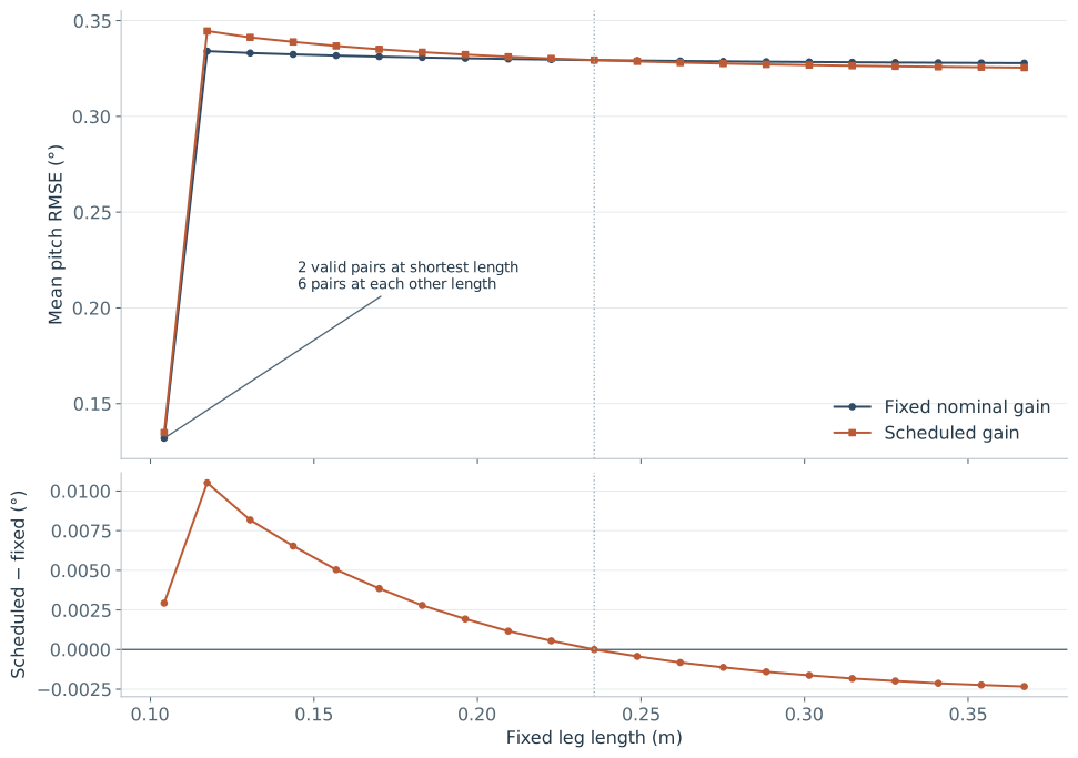
Pitch RMSE and scheduled-minus-fixed difference across 21 fixed leg lengths; scheduling is slightly worse at short lengths and slightly better at long lengths — B1: 252 planned slots, 8 excluded for invalid geometry, 244 valid trajectories and 122 matched pairs. Each point averages 6 pairs, except 0.1042 m with 2 pairs. Positive differences mean higher RMSE with scheduling. B1 report and per-height data ↗

The mean scheduled-minus-fixed RMSE difference across valid pairs was +0.00126°. This grid supports a configuration-dependent tradeoff; it does not establish an overall scheduling advantage.

Disturbance rejection

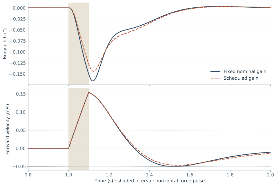
All 36 horizontal-pulse trials completed and recovered. For the longest leg in B2, 0.3146 m, under the largest positive pulse, recovery took 0.447 s with fixed gain and 0.156 s with scheduled gain after the pulse ended. Smaller pulses showed much less difference.

Recorded body-pitch and forward-velocity responses to the largest positive pulse at 0.3146 m, comparing nominal fixed and scheduled gains — B2_H03_V06, both controllers: a positive pulse of 0.20 times nominal half-vehicle weight, applied at 1.0–1.1 s. View window: 0.8–2.0 s of the 6 s record. Dotted lines mark ±0.05 m/s. Raw MAT hashes match the public ledger. B2/B3 protocol and results ↗

Velocity tracking

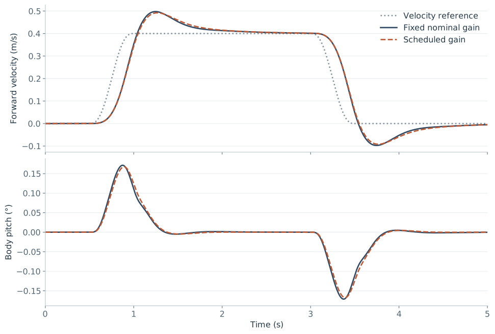
All 24 trials completed and recovered for ±0.2 and ±0.4 m/s commands at three fixed leg lengths. Mean command-interval velocity RMSE was 0.06399 m/s with fixed gain and 0.06386 m/s with scheduled gain. The nearly overlapping curves below illustrate the tracking behavior and body-pitch regulation in this model.

Recorded forward velocity against a plus 0.4 m/s reference and body pitch for both controllers at a fixed 0.3146 m leg length — B3_H03_V04, +0.4 m/s at L₀ = 0.3146 m, both controllers. View window: 0–5 s of the 8 s record. Dashed scheduled and solid fixed responses nearly overlap; the dotted line is the reference. The aggregate RMSE above covers 12 matched conditions.

Model-parameter uncertainty

600 / 600completed and recovered

B4 reused 100 parameter samples across three fixed leg lengths and two controllers, varying mass, inertia, and center-of-mass distance while keeping the controller nominal.

Both controllers recovered in all 300 matched conditions within this designed envelope. The study found no overall recovery-rate advantage for scheduling. B4 report and uncertainty envelope ↗

Simulation protocol & recovery criteria

All studies use ideal sensing, zero noise and delay, a 1 ms controller period, and 0.25 ms RK4 plant substeps. The plots were exported from frozen records; no benchmark was rerun for this page.

B1: 21 leg lengths × 6 initial tilts × 2 controllers, with 8 geometry-excluded slots at the shortest length. Statistics use the 122 jointly valid matched conditions.
B2: three lengths and six signed horizontal-pulse amplitudes, giving 18 matched conditions and 36 trajectories. Recovery time starts at pulse end.
B3: the same three lengths and four signed velocity commands, giving 12 matched conditions and 24 trajectories. RMSE covers the command interval; the reference ramps up, cruises, and returns to rest.
B4: 100 shared parameter samples × 3 lengths × 2 controllers. Each 8 s trajectory starts at +5° pitch. The 600 trajectories form 300 matched conditions.

For the displayed disturbance case, sustained recovery requires |φ| ≤ 1°, |φ̇| ≤ 2°/s, and |ẋᵦ| ≤ 0.05 m/s. Full protocols, denominators, and numerical checks are linked in the reports above.

Validation scope & source evidence

View validation repository Code & model provenance